lumpyspace part 2: weighing the universe

Matter, Constraints, and Spatial Inhomogeneity Link to heading

In my previous post, I explored how a Physics-Informed Neural Network (PINN) could learn the 4D metric tensor of the universe directly from Pantheon+ Supernova data, constrained by the Einstein Field Equations (EFE). The model discovered that extreme spatial anisotropy (a “Cosmological Dipole”) could act as a physical mechanism to mimic Dark Energy in a vacuum universe.

But a vacuum universe is a spherical cow¹. And Supernovae, while excellent standard candles, only give us part of the story. They provide luminosity distances, which act as a proxy for the expansion history of the universe.

From Vacuum to Matter Link to heading

In my first experiment, the vacuum universe was mathematically stable and fit the EFE and supernova data. However, it did so by falling into a contracting regime where space actively shrank ($H < 0$), utilizing extreme shear near the present day as a mathematical cheat code.

While a pure vacuum geometry can technically satisfy the data and the field equations, it is physically unrealistic (our universe actually has stuff in it²). If we want the model to discover a realistic cosmology without falling into contracting local minima, we have to give it the physical vocabulary to do so: Matter.

A Bounded Parameterization for $\Omega_m$ Link to heading

In $\Lambda$CDM cosmology, we might plug in a fixed value like $\Omega_m \approx 0.3$ (about 30% matter, most of which is Dark Matter), a standard assumption validated by the Planck 2018 results. But we want the network to dynamically discover the matter density that best balances the field equations against the data.

So, instead of hardcoding a value, I introduced a trainable matter density parameter, $\Omega_m$, which represents the matter density fraction today.

To prevent the optimizer from taking the lazy way out by bloating $\Omega_m$ to $1.0$ (or higher) to escape into a smooth, homogeneous, matter-heavy metric, we must restrict $\Omega_m$ to the strict physical window $[0.05, 0.3]$³.

We enforce this strict physical window and ensure healthy training dynamics using two techniques:

1. Projected Gradient Descent & Decoupled Optimization Link to heading

Initially, I tried bounding the parameter using smooth mathematical mappings (like sigmoids or double softplus functions). However, these create vanishing gradient zones near the boundaries. It was impossible to tell if the model was even trying to drop $\Omega_m$ as the gradients locked the parameter.

To fix this, we stripped away the mappings and optimized the raw $\Omega_m$ parameter directly, strictly clipping it to $[0.05, 0.3]$ after each step using Projected Gradient Descent (PGD).

But there was another hurdle: the network is a 4-layer, 64-width MLP with thousands of parameters, while $\Omega_m$ is a single scalar. During global norm gradient clipping (optax.clip_by_global_norm), the massive dimensionality of the MLP completely swallowed the scalar’s gradient updates, starving it of any movement. To solve this, we decoupled the optimization.

Using optax.multi_transform, we gave $\Omega_m$ its own dedicated optimizer chain with a 100x boosted learning rate and no global norm clipping. This allowed the matter density to finally participate in the optimization fairly.

I debated the initialization of $\Omega_m$ as it might bias the model a priori to favour Dark Matter or to avoid it. Ultimately, we initialize $\Omega_m$ exactly at the dark matter ceiling of $0.3$. This gives the newborn universe a smooth, mathematically stable runway to fit the expansion data initially, before the EFE residuals might learn to force it to develop spatial inhomogeneities and drag the matter density down to the baryonic floor.

2. The Dynamic Cosmology Coupling Link to heading

In standard cosmological models, one might assume a fixed value for the present-day matter density $\kappa\rho_0$, or assume a static relation like $\kappa\rho_0 = 3\Omega_m H_0^2$ using a constant approximation for the Hubble parameter (e.g., $H_0 \approx 1$). However, since our network dynamically learns the space-time geometry and derives the expansion rate $H(t)$ from the metric itself, assuming a static $H_0$ would introduce a physical inconsistency.

To ensure that the trainable parameter $\Omega_m$ remains physically meaningful and bounded within $[0.05, 0.3]$, we must dynamically couple the energy density $\kappa\rho_0$ to the model’s own derived expansion rate today, $H_{\text{mean}}(1.0)$:

By calculating $H_{\text{mean}}(1.0)$ from the spatial metric components at each training step, this coupling ensures that the matter density parameter $\Omega_m$ we tune is exactly the physical density fraction today. As the universe expands, this pressureless dust field dilutes as a function of the spatial metric determinant ($V \propto \sqrt{\gamma}$). By subtracting this matter field’s Stress-Energy tensor ($T_{\mu\nu}$) from the Einstein tensor ($G_{\mu\nu}$), the physics loss can account for the presence of mass.

Enforcing the Weak Energy Condition Link to heading

When matter density is added to the system, general relativity expects it to behave physically. In comoving coordinates, pressureless dust has a Stress-Energy tensor trace of $T = -\rho$. The contracted Einstein Field Equations then dictate:

Since physical matter density must be non-negative ($\rho \ge 0$)⁴, the local spacetime curvature (the Ricci scalar $R$) must also be non-negative ($R \ge 0$) everywhere.

As the neural network only minimizes EFE residuals, it might attempt an unphysical shortcut, creating regions of negative Ricci curvature ($R < 0$, corresponding to negative energy density) to fit the accelerating expansion of the supernovae without dark energy. To prevent this, I added a squared flat minimum penalty to the EFE loss:

This should enforce the Weak Energy Condition smoothly, leaving physical positive-curvature regions completely unbothered while shutting down any negative-mass cheat codes.

Results and Physical Interpretation Link to heading

With the physical constraints and decoupled optimizer active, we ran the supernova-based training loop with matter. To understand what kind of universe the model discovered, we examine the convergence profile, the directional expansion rates over time, and the spatial maps today ($t=1.0$).

The Optimization Trajectory: Shedding Dark Matter Link to heading

The first question is: how does the network tune the matter density when given the freedom to do so?

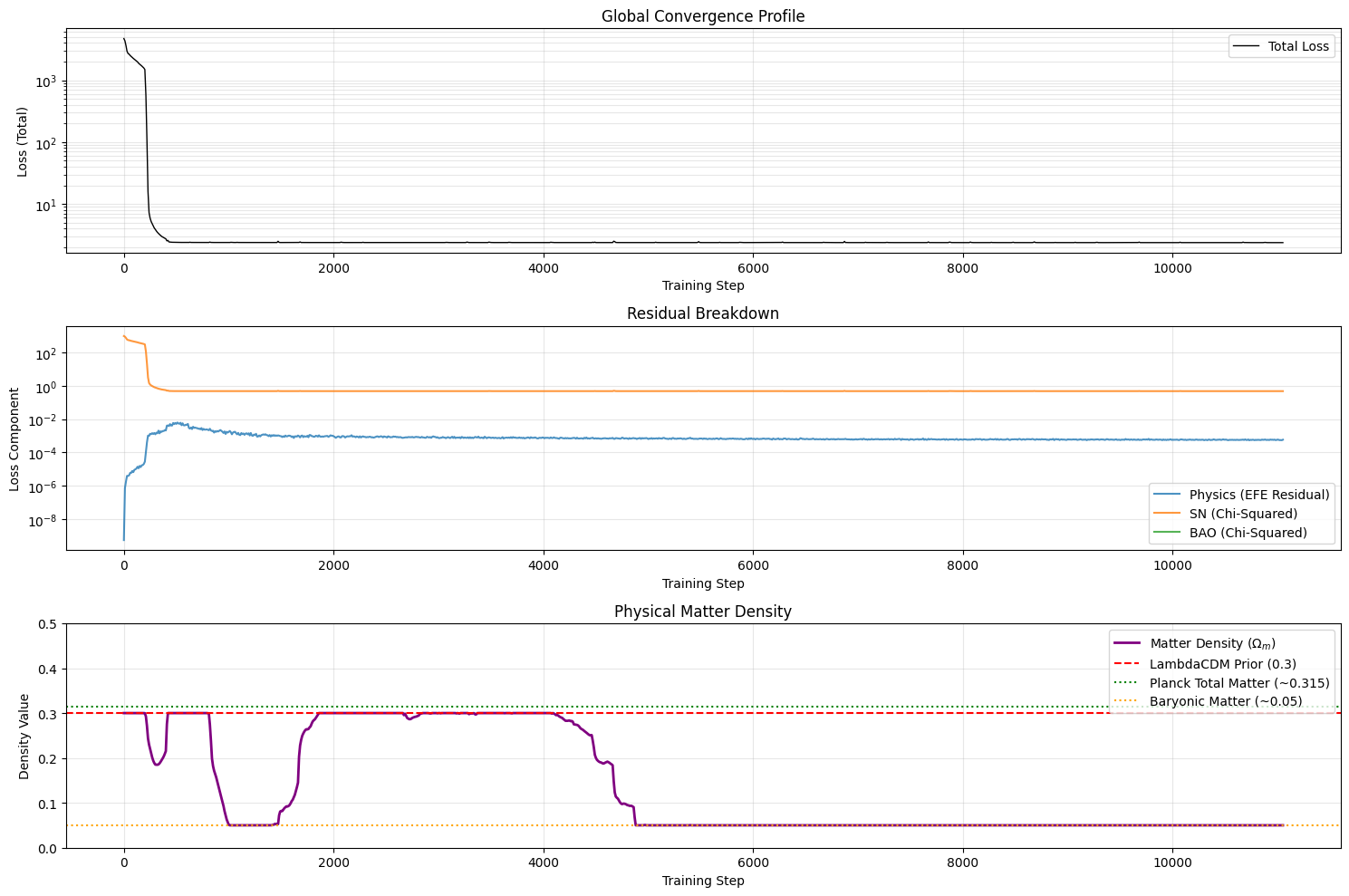
As shown in the bottom panel above, the dynamically optimized $\Omega_m$ parameter plummeted from its $0.3$ initialization (the dark matter ceiling) straight down to the baryonic floor of $\approx 0.05$.

This is a profound result. When the optimizer is forced to reconcile the supernova data with the Einstein Field Equations, it actively rejects the presence of dark matter. It finds that the field equations are much easier to satisfy if the universe is dominated by spatial inhomogeneities rather than a smooth, heavy background of cold dark matter.

Cosmic Shear and Anisotropic Expansion Link to heading

Next, we look at how the expansion rate evolves over coordinate time $t$ (from the early universe at $t=-4.0$ to today at $t=1.0$):

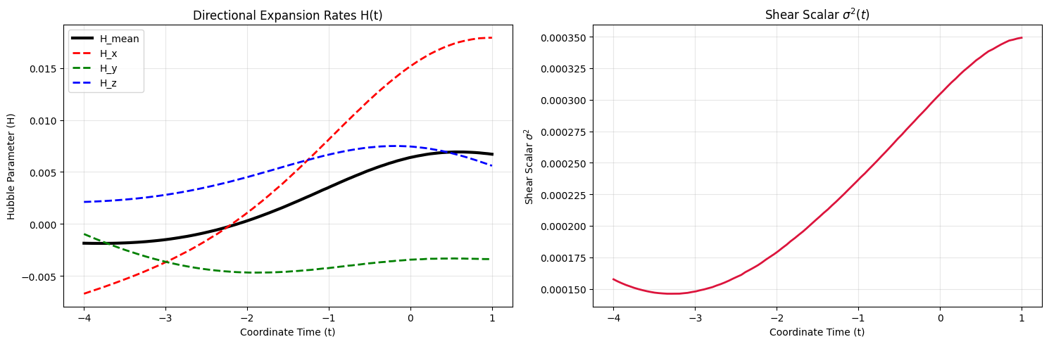
The plots reveal a highly dynamic and anisotropic expansion history:

• Diverging Hubble Rates: In the left panel, the directional expansion rates ($H_x, H_y, H_z$) begin tightly clustered in the early universe, reflecting our isotropic boundary conditions. However, as time progresses, they diverge dramatically. Today ($t=1.0$), the expansion is fast in some directions and slow in others. This is very similar to our previous results though the divergence is gentler and the axes remain closer.
• Late-Time Shear Peak: The right panel shows the shear scalar $\sigma^2(t)$ peaking near the present day. Because shear enters the field equations as an effective energy density term with negative pressure, this late-time spike in shear is precisely the mechanism the network uses to mimic the accelerating expansion rate normally attributed to Dark Energy. Again this is similar to our previous results but with less shear.

Comparison with previous results Link to heading

In the Vacuum Universe ($\rho = 0$)

Under pure General Relativity, a flat, isotropic, vacuum universe cannot accelerate. To force the metric to match the accelerating expansion rate of the Supernovae without Dark Energy, the model had only one mathematical degree of freedom it could exploit: extreme anisotropy (shear). By generating a massive directional shear $\sigma^2$ along our line of sight, the model could stretch the metric and elongate the luminosity distances ($d_L$) to mimic Dark Energy. Shear was the only “sledgehammer” the network had.

In the Universe with Matter ($\rho > 0$)

By introducing a trainable matter density parameter and letting the metric form a spatial curvature gradient (the “Ricci curvature dipole” you see in the 2D maps), the model is no longer forced to rely solely on shear.

Physical Backreaction: Because the metric is now allowed to develop spatial inhomogeneities (the “lumpy” density distribution), the model can exploit the fact that averaging and evolution do not commute in General Relativity:

This spatial lumpiness acts as a physical “backreaction” ($\mathcal{Q}_D$), which naturally alters the expansion history.

Because the spatial density/curvature gradient does a significant portion of the heavy lifting to fit the supernova distances, the optimizer can satisfy the field equations with much milder directional expansion rates and significantly less shear.

Spatial Curvature and Shear Maps Today Link to heading

To visualize the three-dimensional geometry of the universe today, we mapped the shear scalar $\sigma^2$ and the Ricci curvature scalar $R$ across all three principal planes ($x$-$y$, $y$-$z$, and $x$-$z$, with the third coordinate set to 0):

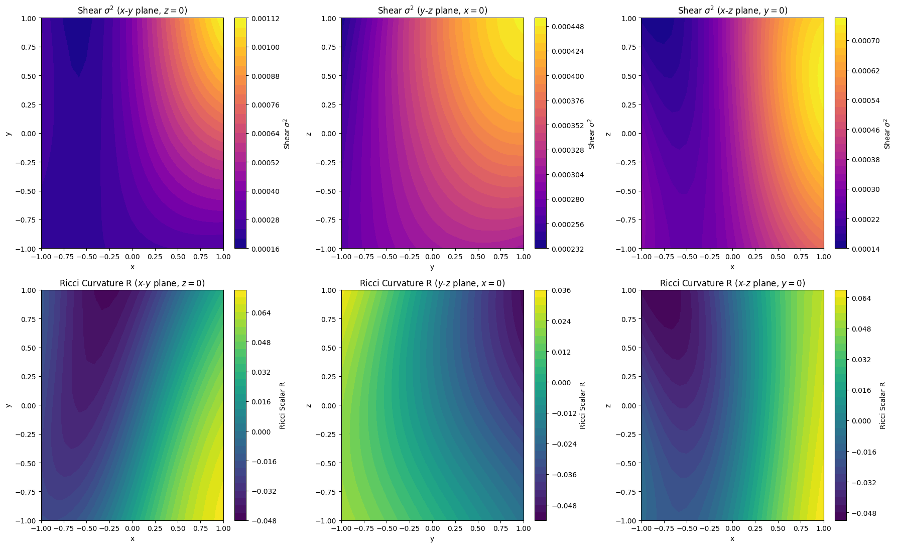
These maps reveal a clear and fascinating picture of spatial inhomogeneity:

• The Curvature Dipole: The Ricci scalar curvature $R$ (bottom row) is not uniform; it forms a distinct spatial gradient (a cosmic dipole) swinging from flat/negative regions to positively curved regions. This represents a massive spatial inhomogeneity (a “lumpy” density distribution) along our line of sight that the model has developed natively from the data.
• Inhomogeneous Shear: The shear scalar $\sigma^2$ (top row) peaks in specific spatial lobes, aligning with the directional expansion gradients.

By letting the matter density and metric evolve freely under pure General Relativity, the network independently demonstrated that the Pantheon+ supernova data can indeed be fit without a cosmological constant (Dark Energy) and without Dark Matter, provided we allow the universe to be inhomogeneous and anisotropic along our line of sight.

By finding a space-time geometry that balances both spatial curvature gradients and directional expansion, the neural network has essentially bypassed the homogeneous Bianchi VII family and independently converged on a solution resembling a Szekeres spacetime, the most general exact inhomogeneous and anisotropic solution to Einstein’s Field Equations.

A final note, and next steps Link to heading

It is worth noting that to a neural network, the laws of physics are merely signs, not cops. Our WEC penalty (and our assumption of zero shear in the early universe) are implemented as soft constraints so the optimizer strikes a mathematical compromise. There is a slight residual negative curvature and non-zero early shear in the final plots as the network balances physical laws against the raw data loss. More on this next…