visualizing m-lab data with bigquery
I recently moved to a new group at Google: M-Lab. The Measurement Lab is a cross-company supported platform for researchers to run network performance experiments against. Every experiment running on M-Lab is open source, and all of the data is also open; stored in Google Cloud Storage and BigQuery.
One of the great things about having all that data open and available in BigQuery is that anyone can come along and find ways to visualize it. There’s a few examples in the Public Data Explorer, but I was feeling inspired1 and wanted to know what it was like for someone coming to M-Lab data fresh.
I decided to build something using HTML5 canvas and JavaScript so those are the versions of the API that I’m using. However, there’s broad language support for the APIs.
OAuth2 authentication Link to heading
This step actually took the longest of the whole process. There are a number of options when it comes to which type of key you need, and how you go about getting one, and the documentation is thorough but not particularly clear. Essentially you need to have view rights for the measurement-lab BigQuery project, and a Client ID created for you by one of the owners. You can ignore any documentation that talks about billing, unless you import the data into your own BigQuery project before running queries against it. However, there’s no need to do that, as a simple email to someone at M-Lab2 you can get a key for your app and view access. This will allow you to run queries at no cost to you.
Once you have a key, it’s time to authorize:
|
|
With this, you should be able to hit the Authorize button, enter a Google account (required for tracking by BigQuery, I believe) and load the BigQuery API library. The Google account you use will have to have accepted the BigQuery terms of service, which involves logging in to the BigQuery site and clicking through the login.
Note, this is a bit of a pain for a multiple-user web application. However, there is the option to set up a server-to-server authorization flow which removes this difficulty. Similarly, I believe native installed applications have a different route for authorization but I haven’t looked into it yet.
Your first query Link to heading
For the purposes of this post, I wanted to get every distinct test that had been run in a month and plot a point at the latitude and longitude of the client’s location. By making the plotted pixel semi-transparent I could use additive blending to make things glow a bit, and easily see areas where multiple tests had run.
I’ll assume you know how to add a canvas to the page and draw to pixels. I’ll focus instead on actually running the query.
|
|
There’s a few things to note here, but the main one is that this is a synchronous call and will timeout and return no results if it takes longer than 45 seconds. It will also return a maximum of 16000 rows. There are ways to remove both of these restrictions which we’ll get to later.
Also, the key to getting values from each row is in the item.f[3].v lines.
The index there comes from the order of fields requested in the SELECT
statement.
Another thing to note is that longitude and latitude could be projected using Mercator or Equirectangular projections.
Removing the restrictions Link to heading
Both the synchronicity of the call and the timeout can be solved by polling for
the query to complete using the jobs.getQueryresults method.
With this change, the code above looks something like:
|
|
As you can see, instead of having a long timeout, we have a short one. When the
callback fires, if the job is not complete, we poll again with the same short
timeout. This continues until the job succeeds (or an error is returned). Note,
this means that even jobs that apparently timeout can remain running and
accessible from the API. If you want to cancel a job you need to delete it using the API.
So what do you get when you run this for 1 million points?
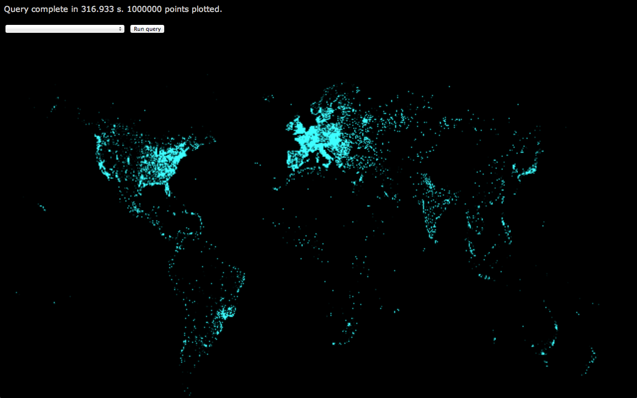
The points are a little fuzzy as I was using CSS to scale up the canvas for a cheap blur effect.
What else? Link to heading
This is pretty enough, but the M-Lab data includes some terrific data regarding the innards of TCP states on client and server machines throughout the tests that are run. This is thanks to the Web100 kernel patches that run on M-Lab server slices. With those, it would be possible to map out areas where congestion signals are more common, or the distribution of receiver window settings. Or try to find correlations between RTT and the many available fields in the schema.
As another simple example, by plotting short RTT in blue, medium RTT in green, and long RTT in red (and removing the blur), you get something like:
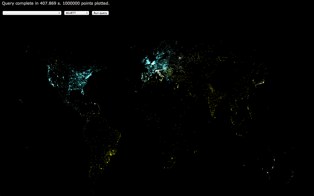
If you look at the full-res version, you can see the clusters of red pixels across India and South East Asia.
This is immediately useful data: Given the number of tests that are run in the area (the density of points), and the long RTT we’re seeing from there, it would make sense to add a few servers in those countries to ensure the data we have on throughput and congestion for that area is not being skewed by long RTT. Similarly, we can feel good about our coverage across Europe and North America, though the less impressive RTT in Canada should be investigated.
More? Link to heading
Almost certainly, but I’m out of time on this little weekend project hacked together between jaunts around Boston. Someone smarter than me can probably combine the fields in the m_lab table schema in ways I haven’t considered and draw out interesting information. Similarly, the live version3 could support zooming and panning of the map, and more flexibility in setting the query from the UI.
Lastly, if you want to start playing around with >630TB of network performance data, let me know and I’ll see what I can do.
-
Hint: Try dominic at measurementlab dot net. [Ed: don’t. the email is a dead one] ↩︎
-
I did mention that there’s a live version right? [Ed: sadly lost, like tears in rain] ↩︎