lumpyspace part 3: calling the physics cops

Transitioning from Soft Penalties to Hard Constraints Link to heading

In my previous post, I introduced a trainable matter density parameter $\Omega_m$ and a soft penalty to enforce the Weak Energy Condition (WEC), which requires the local curvature, the Ricci scalar $R$, to be non-negative ($R \ge 0$) everywhere. The model responded by rejecting Dark Matter entirely, driving $\Omega_m$ straight to the baryonic floor of $\approx 0.05$, and fit the Pantheon+ supernovae using a spatial curvature dipole and anisotropic shear.

But I also noted a caveat: The WEC was implemented as a soft, quadratic penalty in the loss function so the optimizer struck a mathematical compromise: It allowed a slight residual negative curvature ($R < 0$) and non-zero early-universe shear to help fit the raw supernova distances.

To take this inhomogeneous model seriously, we cannot allow the network to compromise on general relativity. The physics must be a hard boundary. So, it’s time to call the physics cops.

The Vanishing Gradient of Soft Constraints Link to heading

Our initial WEC penalty was defined using a standard squared minimum:

Mathematically, this seems reasonable. If $R \ge 0$, the loss is zero. If $R < 0$, the penalty scales quadratically.

However, this formulation has a fatal flaw at the boundary: the gradient of this penalty is proportional to $2 \cdot \min(R, 0.0)$. As the curvature $R$ approaches the boundary from the negative side ($R \to 0^-$), the gradient vanishes. The “restorative force” pulling the model back into the physical regime becomes weaker and weaker the closer it gets to satisfying the law, allowing the network to comfortably park itself in a state of mild violation.

To fix this, we made two key changes:

Linear Violation Penalty Link to heading

We changed the penalty term from quadratic to linear:

Because this function is linear for negative values, its gradient is a constant non-zero step function. The network receives the exact same, strong restorative gradient regardless of whether it is slightly violating the WEC or massively violating it.

The Augmented Lagrangian Method Link to heading

Instead of relying on a static, soft weight that the network can easily scale away, we treat the energy condition as a true hard inequality constraint. The total loss now incorporates a dynamic Lagrange multiplier ($\lambda_{\text{WEC}}$) alongside a quadratic penalty term:

Inside our JIT-compiled training loop, the Lagrange multiplier dynamically accumulates at every single optimization step based on the remaining WEC violation:

If the network attempts to violate the WEC, the multiplier $\lambda_{\text{WEC}}$ climbs higher and higher, acting as a feedback loop that increases the cost of violation until the network is forced back into compliance.

The Lazy Optimizer Trap: Why We Avoided Self-Adaptive Weights Link to heading

It’s worth mentioning an architectural trap we fell into while trying to balance these competing physical constraints. We attempted to use “Homoscedastic Uncertainty Weighting”: a popular PINN method that makes the loss weights ($\sigma_i$) learnable parameters, dynamically balancing gradients by minimizing $\sum \left( \frac{\mathcal{L}_i}{2 \sigma_i^2} + \log \sigma_i \right)$.

While elegant, I discovered that it creates a “Lazy Optimizer” problem. The Einstein Field Equations are a highly rigid, non-linear system, so finding a metric that satisfies them is difficult¹. Faced with a high physics loss early in training, the optimizer found it mathematically cheaper to just drive $\sigma \to \infty$ to artificially zero out the effective loss, rather than actually solving the differential equations! This completely stalled the training. I reverted back to hand-tuned static hyperparameters and the Augmented Lagrangian, which act as unyielding constraints that force the network to solve the physics.

The Spatial Curriculum: Learned 4D Spatial Weights Link to heading

With homoscedastic uncertainty weighting failing globally across different loss components, I realized that the core issue wasn’t balancing the types of physics, but balancing the locations of the physics.

Because our metric has discovered an inhomogeneous spatial curvature dipole, the differential equations are significantly harder to satisfy in some regions of space-time than others. Specifically, the gradients in the high-redshift past ($t \approx -3.0$) are massive compared to the local universe where the supernova data sits ($t > -1.5$). The model was struggling to converge on the Weak Energy Condition because the gradients were dominated by these boundary regions.

To solve this, I introduced a tiny, auxiliary neural network: the spatial_weight_net. This network takes the full 4D spacetime coordinate $(t, x, y, z)$ and outputs a single scalar attention weight $W(t, x, y, z)$.

We then apply the homoscedastic uncertainty formula locally at every spatial point:

This acts as a completely automated spatial curriculum. The network learns to dynamically scale down the loss in regions of extreme gradient magnitude by increasing $W$ locally. As it solves the “easy” zones, it naturally decreases $W$ in the harder zones to focus its attention there.

Applying the Curriculum to the Physics Cops Link to heading

To ensure the Augmented Lagrangian (AL) penalty for the WEC is not dwarfed by the massive gradients of the supernova data, we integrate the point-wise AL penalty directly into the spatial curriculum.

By computing the total physical error (EFE residual + AL penalty) before applying the $e^{-2W}$ attention map, the network can massively amplify the AL penalty in the exact regions where the WEC is violated. This ensures that the hard physics constraint is optimized effectively, forcing the network to solve the complex spatial geometry systematically rather than relying on Dark Matter.

Results Link to heading

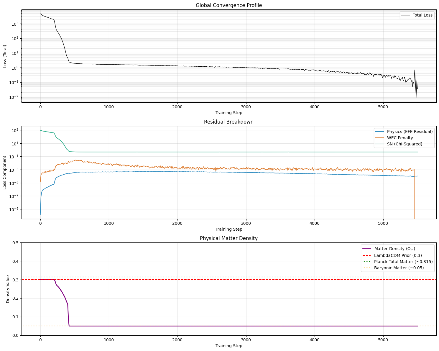
During training, the WEC loss ($\mathcal{L}_{\text{WEC}}$) eventually dropped, though it took quite a bit more training than previous runs. As you can see in the loss profile below, right around step 5400, the telemetry logged a value of exactly 0.000000e+00.

Because the WEC loss is the average of the violation over the entire coordinate grid, hitting exactly zero means the Ricci scalar $R \ge 0$ at every single coordinate point evaluated. The feedback loop worked as intended. When the model drifted slightly, the accumulated Lagrange multiplier responded by pulling it back down to zero.

Visualizing the Spatial Curvature Today Link to heading

We generated fresh 2D spatial maps of the Ricci scalar curvature today ($t = 1.0$):

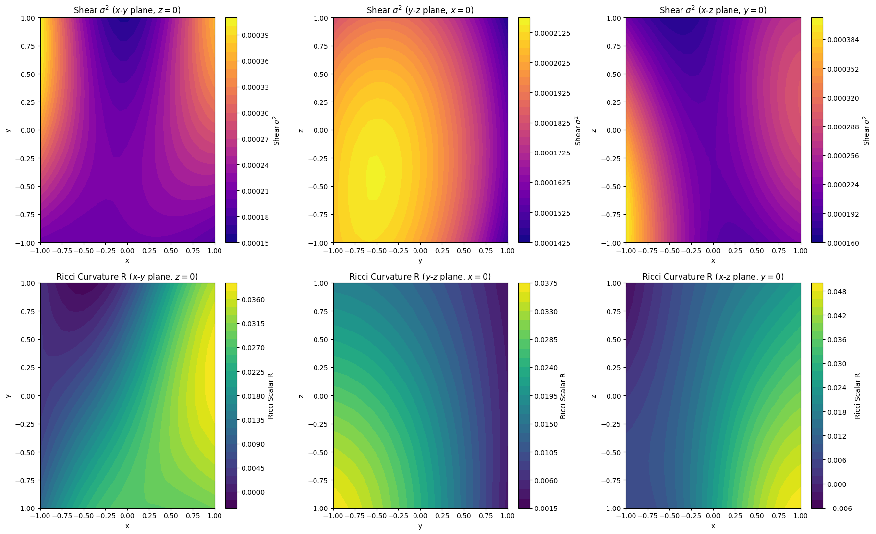
Looking at the bottom row (Ricci Curvature $R$), the colorbars show a clear improvement. The negative-mass shortcuts have been largely eliminated. (You might notice a microscopic -0.006 minimum in the $x$-$z$ plane colorbar despite the loss logging exactly zero. This is a PINN quirk: we enforce on a finite set of random collocation points. Between those points, the continuous neural network can still “ripple” slightly below zero, but it’s tightly bounded on a macroscopic scale!).

And once again, $\Omega_m$ was driven straight to the baryonic floor of 0.05. Even under strict general relativity, the universe rejects the homogeneous Dark Matter assumption.

Interpreting the Inhomogeneous Geometry Link to heading

With the spatial curriculum active, we can visualize the complex, valid spacetime geometry the network has discovered. Check out these 3D surface plots of the Ricci curvature:

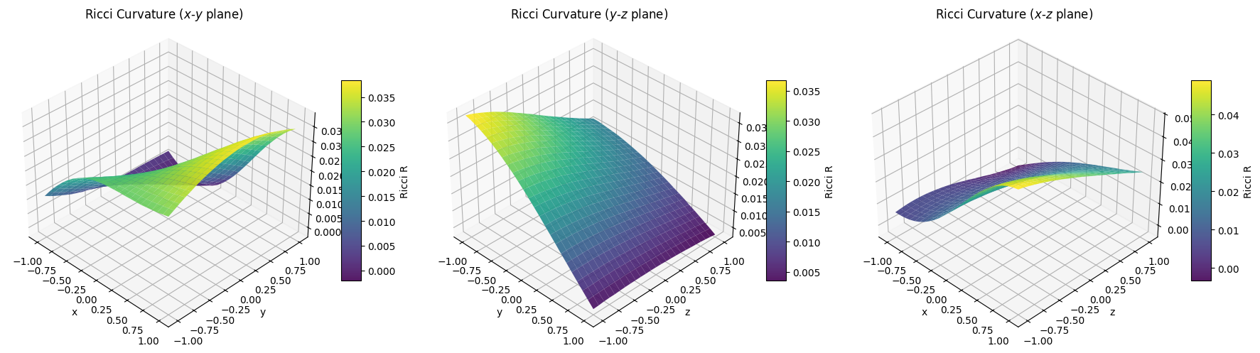
The network hasn’t just found a simple gradient; it has discovered a saddle-like topology in the spatial curvature. The curvature bends and warps dynamically across the $x$-$y$, $y$-$z$, and $x$-$z$ planes, adapting to fit the anisotropic supernova distances while being bounded by the WEC penalty pulling it up from the zero-plane. This inhomogeneous structure demonstrates how the model can explain the data without relying on Dark Matter.

The Next Frontier: The past drifts Link to heading

Enforcing the laws of physics as a hard boundary has solved our negative mass problem, but it has revealed a new, fascinating artifact in the early universe ($t = -4.0$):

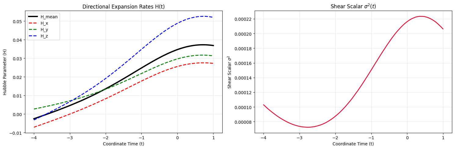
In the left panel, the directional Hubble parameters ($H(t)$) start near zero or slightly negative in the past ($t = -4.0$). In the right panel, the shear scalar ($\sigma^2(t)$) bends back up to $\approx 1 \times 10^{-4}$ at $t = -4.0$.

As the matter density is so low ($\Omega_m = 0.05$), the universe in the past ($t \in [-4.0, -1.5]$) behaves like a vacuum. Without a heavy background of matter to drive cosmic expansion and deceleration, and because we have no observational supernova data in the far past (Supernovae only go up to $z \approx 2.3$, or $t \approx -1.5$), the neural network’s extrapolation is free to drift. Under pure vacuum field equations, it drifts into a static/contracting past with positive shear.

But the Cosmic Microwave Background (CMB) tells us that the early universe ($z \approx 1100$, or $t \ll -4.0$) was highly isotropic and expanding.

What’s Next: Enforcing the CMB Constraints in the Early Universe Link to heading

To address this, we must introduce the final pieces of the physical puzzle: a three-part Early-Universe Prior applied at $t \le -3.0$. To ensure our model merges smoothly with standard FLRW cosmology at high redshifts and matches the stunning uniformity of the Cosmic Microwave Background, we will penalize three things in the early universe:

1. Negative Expansion ($H_{\text{mean}} < 0$): The universe must be expanding.
2. Anisotropic Shear ($\sigma^2 > 0$): The expansion must be isotropic in all directions.
3. Spatial Gradients ($\sum (\partial_i g_{\mu\nu})^2 > 0$): We must enforce spatial homogeneity to prevent the network from hiding massive curvature dipoles in the early universe, which would violently conflict with the $10^{-5}$ density perturbations of the CMB.

By anchoring the network with these physical boundary conditions in the deep past, the Einstein Field Equations will naturally propagate that smoothness forward, preventing the unphysical “past drifts” without us having to explicitly simulate complex recombination plasma dynamics.

Stay tuned!