lumpyspace part 4

A Confession Link to heading

In my previous post, I explained that we had implemented an Augmented Lagrangian (AL) method to strictly enforce the Weak Energy Condition (WEC). I shared monitoring showing the WEC loss dropping to exactly 0.000000e+00.

However, it turns out we had fallen victim to a silent scoping bug inside the JAX @eqx.filter_jit compiler.

To capture static hyperparameters (like w_efe, w_sn) without passing them explicitly, we wrote our loss_fn as an internal closure inside the compiled step function. This is a common JAX pattern. However, the Augmented Lagrangian multiplier ($\lambda_{\text{WEC}}$) is a dynamic array that changes every single optimization step.

We dutifully passed the dynamic lambda_wec array into the step function signature. But inside the loss_fn closure, we accidentally referenced the python variable lambda_wec_val from the outer training scope—which had been initialized to exactly 0.0 before the training loop started.

When JAX traces a function for the first time to compile it into an XLA graph, it captures outer-scope variables as static constants. JAX saw lambda_wec_val = 0.0 and hardcoded it.

While our outer python loop was happily calculating the AL multiplier and printing updated $\lambda$ values to the terminal, the neural network inside the JIT-compiled graph was blindly calculating 0.0 * violation on every single step. The network never felt the compounding Augmented Lagrangian pressure at all!

The “compliance” we saw in the previous post was simply the network reacting to the standard quadratic penalty ($\frac{\mu}{2} \text{violation}^2$). We had accidentally degraded our advanced AL method into a basic Quadratic Penalty Method.

We have since patched the scoping bug. The network will now feel the true pressure of $\lambda$.

Re-balancing the Sampling Tension Link to heading

To ensure the network didn’t use unobserved coordinate gaps to hide singularities or workarounds to the constraints, I increased our spacetime sampling to $t=[-3.9, 1.0]$ and bumped our grid sampling to 1000 points. I also re-balanced the grid to a strict 800/200 split. This anchors the active Supernova region with $\approx 228$ points per unit, while still giving the deep past enough resolution ($\approx 133$ points per unit) to prevent mathematical aliasing.

The “Shock Absorber”: Adaptive Penalty Scheduling Link to heading

Even with the AL multiplier un-frozen and the true $\lambda_{\text{WEC}}$ penalty applied, we discovered a new failure mode: the “Lazy Optimizer.” If the penalty parameter $\mu$ is fixed, a deep neural network will often find a local minimum where it just balances the data loss against the physical penalty instead of driving the physical violation to absolute zero.

To combat this, we completely encapsulated the Augmented Lagrangian state and implemented an Adaptive Penalty Scheduler.

By tracking an Exponential Moving Average (EMA) of the constraint violation, the scheduler acts like a mathematical shock absorber:

• When the network is making good progress (the EMA is dropping), the scheduler completely backs off and lets the gradients descend naturally.
• When the network stalls or tries to cheat (the EMA fails to drop by at least 10% over 500 steps), the scheduler violently scales the penalty weight $\mu$ by a factor of 10.

If the network stalls for 500 steps, the penalty rockets from $1.0 \rightarrow 10.0 \rightarrow 100.0 \rightarrow 1,000.0 \rightarrow 10,000.0$. This builds a massive brick wall that forces the optimizer right back into physical reality the second it gets lazy.

The Results Link to heading

First, let’s look at the convergence and physical parameters:

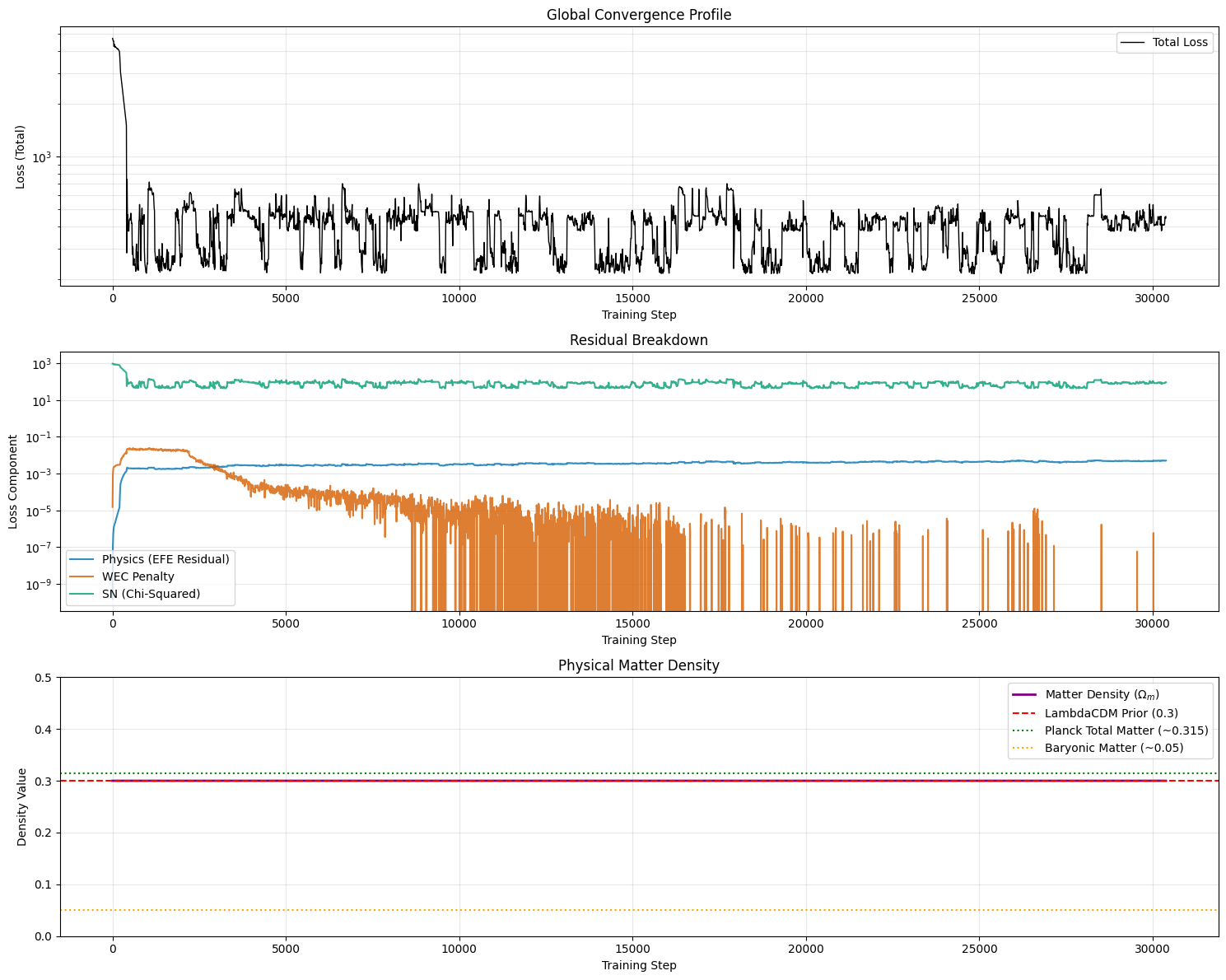
The Augmented Lagrangian method performed as expected though it took a lot longer to get there than previously, due to the sampling of the longer time-range. The WEC penalty (l_wec) hit a stable 0.000000e+00 however, look at the bottom panel. The matter density $\Omega_m$ is stuck at $0.3$. It did not drop to the baryonic floor like it did in previous runs.

In our earlier runs, the sparse sampling allowed the network to hide small regions of negative energy between evaluation points. The network used this negative energy to generate the acceleration required to fit the Supernova data, which allowed it to drop $\Omega_m$. Now that the grid is densely sampled down to $t=-3.9$, the network is fully constrained by the WEC everywhere.

Without negative energy or a Cosmological Constant, how is it fitting the Supernovae? Let’s check the kinematics:

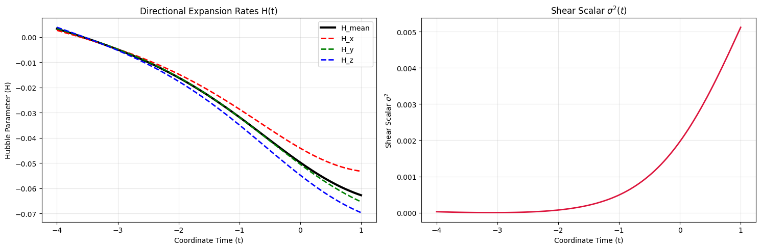
The network has found a mathematically valid but physically backward solution. It describes a collapsing universe.

To fit the Supernova data while collapsing, the network discovered a mathematical loophole: it uses severe time-dilation (a cosmological gravitational well) to perfectly mimic the redshift of an expanding universe!

We know our actual universe is not doing this thanks to Big Bang Nucleosynthesis (which requires true spatial compression in the past) and structure formation dynamics. But the Einstein Field Equations are time-reversible and supernova data alone cannot break this degeneracy, so the neural network drifted into a local minimum where the universe is contracting ($H_{\text{mean}} < 0$).

The Real Next Frontier: Anchoring the Early Universe Link to heading

These results show that we cannot rely on the Einstein Field Equations alone to define the arrow of time. This brings us to the CMB Priors.

By anchoring the deep past with explicit penalties against negative expansion and anisotropic shear, we can break the time-reversal symmetry and force the network into an expanding phase. This will test whether an inhomogeneous, expanding universe can explain the Supernova data without Dark Matter.

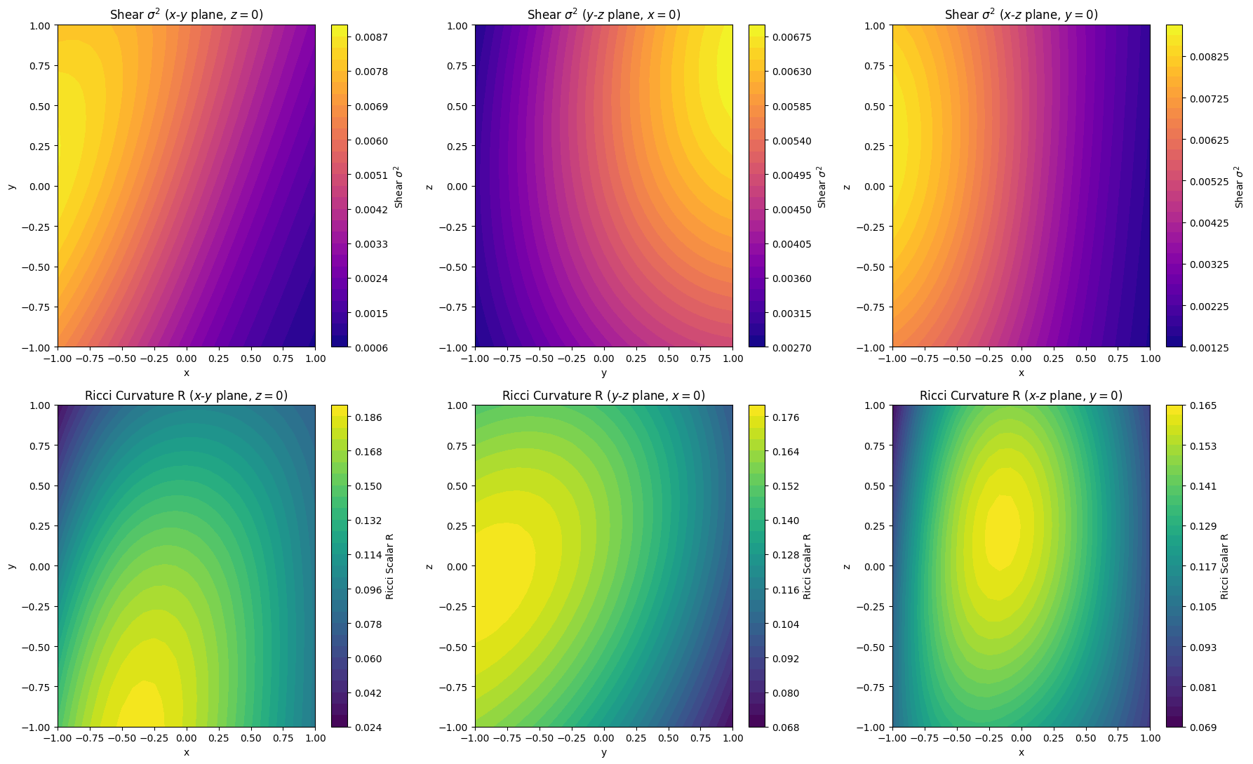
Without observational data to guide it, the time-reversible nature of general relativity allows the neural network to mathematically drift into a contracting phase ($H < 0$) with high spatial shear.

But we do have observational data about the deep past: the Cosmic Microwave Background (CMB). The CMB guarantees that at high redshifts, the universe was isotropic, highly homogeneous, and actively expanding.

Implementing the CMB Constraints Link to heading

At the deepest boundary of our computational domain ($t \in [-4.0, -3.9]$), we will deploy our (now fully functional) Augmented Lagrangian method to penalize three specific geometric deviations:

1. Expansion Rate ($H_{\text{mean}} < 0$): We explicitly penalize negative expansion. This breaks the time-reversal symmetry of the Einstein Field Equations and forces the network out of the “contracting universe” local minimum.
2. Anisotropic Shear ($\sigma^2 > 0$): We penalize any non-zero shear scalar, forcing the early universe to be perfectly isotropic.
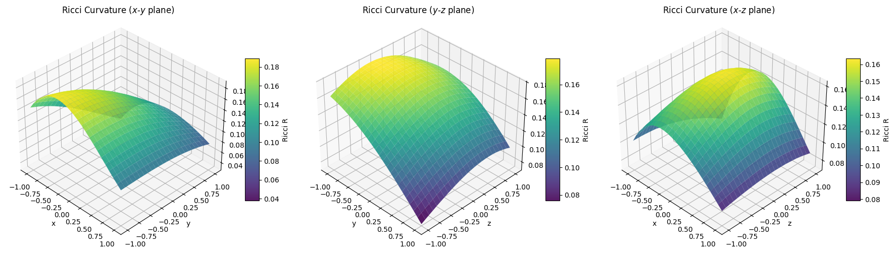
3. Spatial Gradients: We penalize the spatial derivatives of the metric components ($\sum (\partial_i g_{\mu\nu})^2 > 0$), forcing the early universe to be smooth and homogeneous, matching the $10^{-5}$ density perturbations of the CMB.

By anchoring the deep past with these three CMB priors, the Einstein Field Equations will naturally propagate that smooth, expanding geometry forward in time. This forces the neural network to solve the complex, inhomogeneous Supernova geometry in the local universe without relying on bizarre artifacts in the unobserved past.