lumpyspace part 6: the volume knob
Matter, and the early universe Link to heading
At the end of my last post, the supernova data was finally reaching the network, and the geometry it fitted that data with had three problems. The mean expansion rate today was negative, about $-0.0025$ in code units against an observed $H_0$ of about $0.24$. The supernova redshift came almost entirely from the lapse $\sqrt{|g_{00}|}$, a gravitational potential centred on the observer, and not from expansion. And at the boundary where we apply the Cosmic Microwave Background (CMB) constraints, the shear was between two-thirds of and twice the expansion rate, where the CMB bounds it below $10^{-5}$.
This run made two changes. The matter density is now trained as an absolute density, bounded by the observed baryon and total matter densities, where before it was derived from the expansion rate. And the CMB constraints now measure shear and contraction as fractions of the expansion rate, and metric variation as a perturbation amplitude, each held to $10^{-5}$ from the first step. Both changes worked. The run also showed that the spatial weighting introduced in part 3, a learned weight on the field-equation and energy-condition losses at each point, had been scaling those losses down by factors of up to $10^6$.
An absolute matter density Link to heading
Until now the matter density was tied to the expansion rate:
$$\kappa\rho_0 = 3\,\Omega_m H^2$$A universe with $H \approx 0$ had no matter in it, and so no reason to expand. That was the hole the network sat in at the end of part 5.
So the trained parameter is now the absolute density $\kappa\rho_0$, bounded between two physical densities: the baryons, which Big Bang nucleosynthesis fixes from deuterium abundances and the CMB temperature, and the total matter. Neither bound refers to $H_0$. $\Omega_m$ becomes something the fit reports instead of something we clip.
With a density bounded away from zero, flat empty space no longer satisfies the field equations. The time-time component of the Einstein Field Equations (EFE) is the Friedmann constraint:
$$3H^2 - \sigma^2 + \tfrac{1}{2}{}^3R = \kappa\rho$$Put matter on the right and something on the left has to balance it: expansion ($H$), shear ($\sigma$), or spatial curvature (${}^3R$).
Holding the early universe to the CMB Link to heading
The CMB constraints from part 5 were too weak to matter, for three reasons. They squared their violations, so a miss of $10^{-3}$ registered as $10^{-6}$. Their tolerances were absolute numbers, when the CMB constrains shear and contraction relative to the expansion rate. And they started at a weight of 1, gaining strength only when the adaptive scheduler bumped them, once every thousand steps.
Before rewriting them, I asked whether they should stay Augmented Lagrangian constraints at all. They should. Part 3 showed that a fixed-weight penalty lets the network keep a little violation and pay the price; the Lagrange multiplier $\lambda$ keeps raising that price until the violation is gone. Part 4 showed that a fixed penalty weight settles into the same compromise one level up, which is what the adaptive scheduler is for.
What changed is how they measure, and how hard they start:
- Shear as $\sigma^2 / (H^2 + \sigma^2)$, which is $(\sigma/H)^2$ while the shear is small and approaches 1 when shear dominates.
- Contraction as the share of the squared directional expansion rates that is contraction, between 0 and 1.
- Homogeneity as the amplitude of the metric’s spatial variation per Gpc.
Each is a linear hinge at the CMB’s $10^{-5}$, starting at a weight where a full violation costs about as much as a mediocre supernova fit. We started weak before because a physics-heavy start used to collapse the network into flat, empty Minkowski space, which satisfies every physics term for free. With an absolute matter density, Minkowski isn’t free any more.
The energy condition stays on part 3’s linear form, $\max(0, -R)$, at part 3’s starting weight of 10. I did try turning it into a fraction like the others, and learned why part 3 made it linear: the curvature here is a hundred times the matter term, so the fraction sat at 1 wherever $R < 0$ and stopped pushing exactly where the violation was largest.
The results Link to heading
The run went for 49,000 steps. Everything below comes from its best checkpoint, at step 38,023.
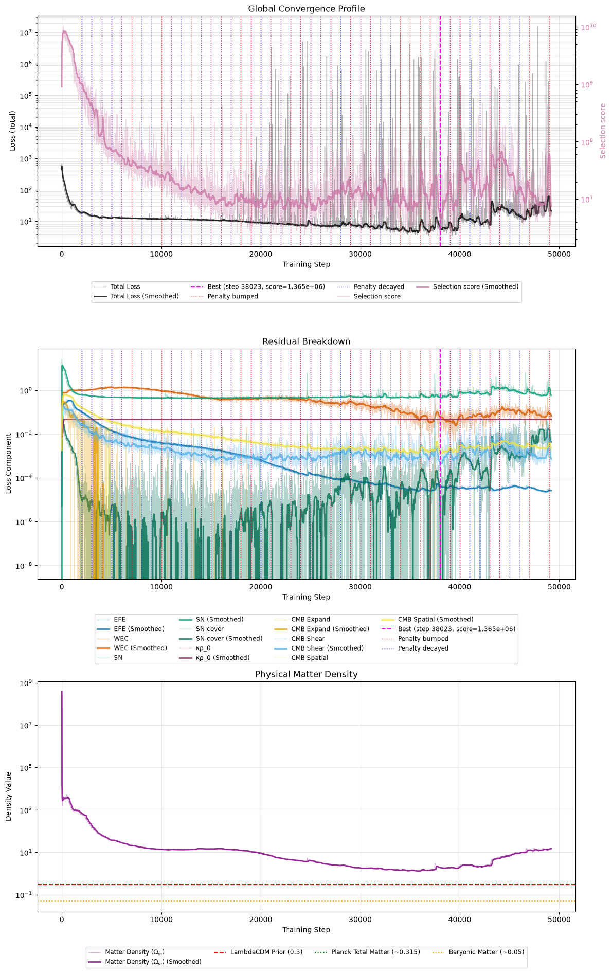
Three things stand out in the residuals. The CMB terms (yellow, gold and light blue) fall straight away. The energy condition (dark orange) sits near 1 for the first ten thousand steps, through every penalty bump. And the field-equation residual (blue) keeps falling for the entire run, by more than three orders of magnitude.
The early universe, fixed Link to heading
The CMB constraints worked at their starting weight, before the scheduler had touched anything. Within a few thousand steps the boundary at $t = -4$ was expanding on every axis at nearly the same rate, and it stayed that way.
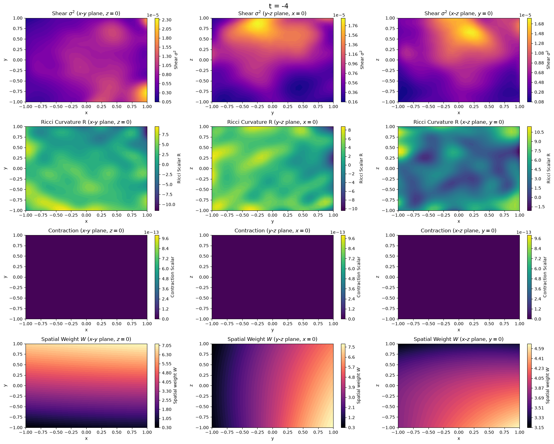
For comparison, here’s the same slice at the end of part 5:
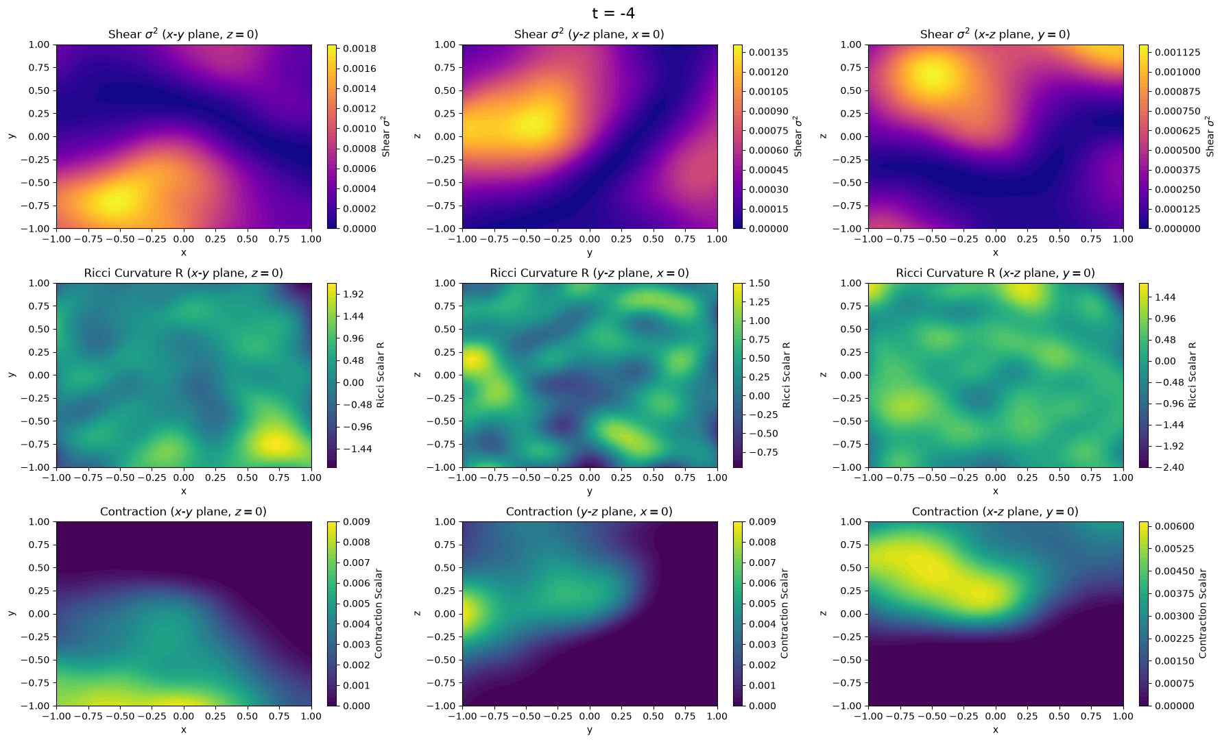
- No contraction anywhere. The contraction maps are flat zero, and the contraction loss reads exactly zero on almost every step after the first five thousand.
- Shear about 1% of the expansion rate. In part 5 it was between two-thirds of and twice the expansion rate at the boundary.
- The metric’s spatial variation fell from about $0.5$ to about $0.001$ per Gpc.
That’s still a long way from the CMB’s $10^{-5}$, and shear is now nearly all of what keeps the score from improving. But the early universe now looks like an early universe: smooth, isotropic, and expanding.
Expansion Link to heading
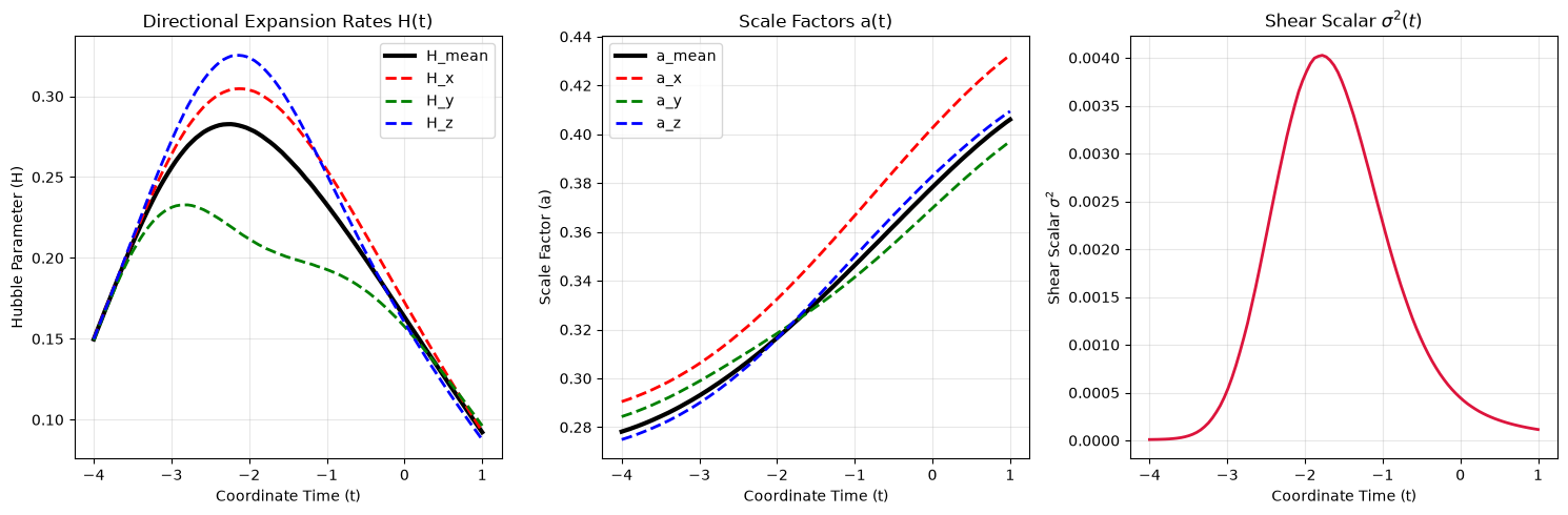
For the first time in this project, the universe expands at a meaningful fraction of the observed rate. Along the observer’s line, every axis expands throughout the history, the mean scale factor grows by 46%, and $H$ today is $0.092$ in code units: 39% of 70 km s⁻¹ Mpc⁻¹. At its peak, around step 35,000, it reached 45%.
The matter density went straight to its ceiling, the total observed matter, within the first few hundred steps and stayed there. So the falling $\Omega_m$ in the bottom panel of the loss chart is $H$ rising: $\Omega_m$ is matter relative to the critical density $3H^2/\kappa$.
The field equations say what it would take to get the rest of the way. Their time-time component holds at every point, with no assumption of flatness or isotropy:
$$3H^2 = \kappa\rho + \sigma^2 - \tfrac{1}{2}{}^3R$$At the observed $H_0$, the left-hand side is about $0.16$ in code units. Matter at its observed maximum supplies $\kappa\rho \approx 0.047$ of that, about 29%. The other 71% has to come from shear ($\sigma^2$) or negative spatial curvature (${}^3R < 0$). $\Lambda\text{CDM}$ sets both to zero and fills the gap with a cosmological constant. Here the network has only the geometry to fill it with, and whether the geometry can is the question this project exists to ask.
A shape that shouldn’t exist Link to heading
Look at the shape of $H(t)$. It rises from the boundary to a peak around $t \approx -2.2$, then falls into today.
The falling half is ordinary deceleration. The rising half shouldn’t be there. Raychaudhuri’s equation gives the rate of change of the matter’s expansion $\theta$:
$$\frac{d\theta}{d\tau} = -\tfrac{1}{3}\theta^2 - \sigma^2 + \omega^2 - R_{\mu\nu}u^\mu u^\nu + \nabla_\mu a^\mu$$For pressureless dust that satisfies the field equations, $R_{\mu\nu}u^\mu u^\nu = \tfrac{1}{2}\kappa\rho > 0$, and the dust falls freely, so $a^\mu = 0$. That leaves rotation, $\omega^2$, as the only term that can push the expansion rate up, and it would have to outweigh everything else put together. The shift terms in our metric do allow the matter to rotate, and I haven’t measured how much. The simpler reading is that a rising $H$ marks a stretch of history where the field equations don’t hold.
Keep that in mind. It comes back below.
Today Link to heading
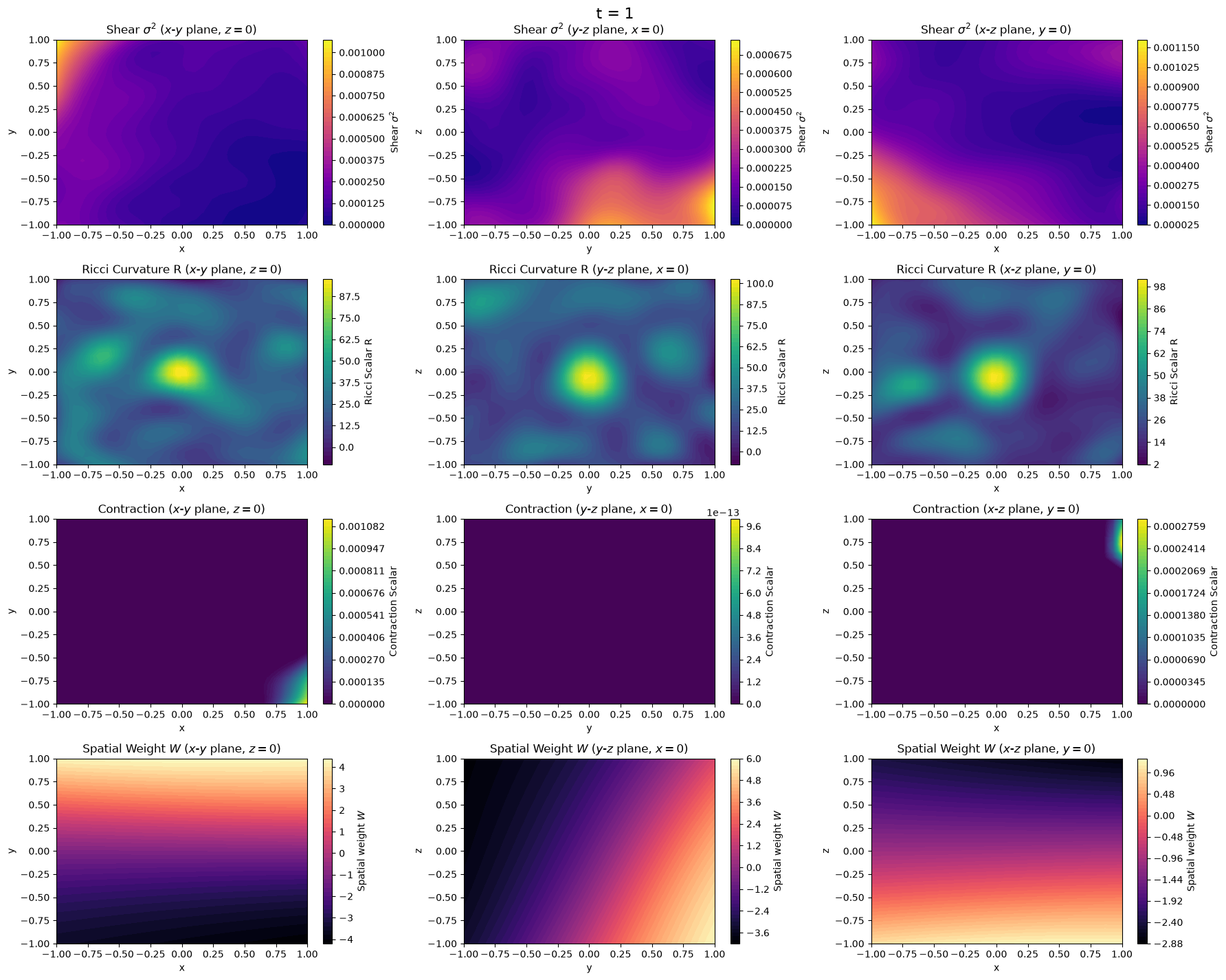
The CMB constraints act at $t = -4$. Today, only the field equations act on the geometry, and the slice shows it. The observer still sits on a lump of positive curvature, $R \approx +100$, thousands of times the matter term. Part 5 found the same lump, smaller. It’s about $0.15$ across, so on any step only a couple of the thousand points where we check the field equations land in it. It’s also exactly where every light ray starts, which makes it the obvious suspect for where the supernova redshift is really coming from.
The volume knob Link to heading
One constraint behaved differently from the others. The energy condition sat near 1 for ten thousand steps while the scheduler raised its weight a thousandfold and its multiplier climbed past 60,000. At one point the multiplier alone should have added about 29,000 to the loss; the total loss moved from 12.3 to 12.9. The CMB contraction constraint, at a weight of 100, had fallen by more than half in its first thousand steps.
Something was absorbing the penalty, and I’d built it.
The lazy optimizer, again Link to heading
In part 3 we tried homoscedastic uncertainty weighting, which gives each loss term a learnable weight $W$ and minimises
$$\tfrac{1}{2} e^{-2W} L + W$$The network drove $W \to \infty$ to switch the physics off, the “Lazy Optimizer”, and we dropped it.
The very next section of part 3 brought the same formula back, one point at a time. The spatial curriculum is a small network that outputs $W(t, x, y, z)$ at every point where we check the field equations, and the physics there costs $\tfrac{1}{2} e^{-2W} L + W$. The reasoning was that the trouble lay in balancing locations, not loss types. Then, so the energy condition wouldn’t be “dwarfed”, we put its penalty inside the same weighting.
Minimise that cost over $W$ and the best weight is $W = \tfrac{1}{2}\ln L$. It rises with $L$: wherever the physics is badly violated, the network turns it down. The gradient reaching the metric becomes $\tfrac{1}{2},\partial \ln L$, and multiplying $L$ by any constant (a bigger weight, a bigger $\lambda$) leaves $\partial \ln L$ unchanged. Every escalation the scheduler makes is cancelled. The CMB constraints sit outside the weighting, which is why they responded and the energy condition didn’t.
Looking at $W$ Link to heading
$W$ was computed on every step and never logged or plotted. So I plotted it.
Sixteen thousand steps into the run, $W$ was between 3 and 6 almost everywhere, at every time. The physics at each point is multiplied by $\tfrac{1}{2} e^{-2W}$, so the field equations and the energy condition were counting for between a thousandth and a millionth of their face value across the whole of spacetime. The curriculum was supposed to turn down the stiff early universe and ease off as it converged. What it had learned was a single smooth tilt across space, the same at $t = -4$ as today.
The size fit the mechanism. $W \approx 4$ means $L \approx e^8 \approx 3000$ at a point, far above the field-equation residual of about $0.002$, and right where the energy condition’s multiplier, times its violations, lands. The field equations share that $L$, so they were being divided by it too. The energy condition’s penalty was drowning out the field equations.
Then it turned around. The energy condition’s violations kept shrinking as the rest of the geometry smoothed out, down to almost nothing by step 39,000. With them gone, $L$ at most points dropped to the scale of the field-equation residual, and $W = \tfrac{1}{2}\ln L$ followed it below zero.
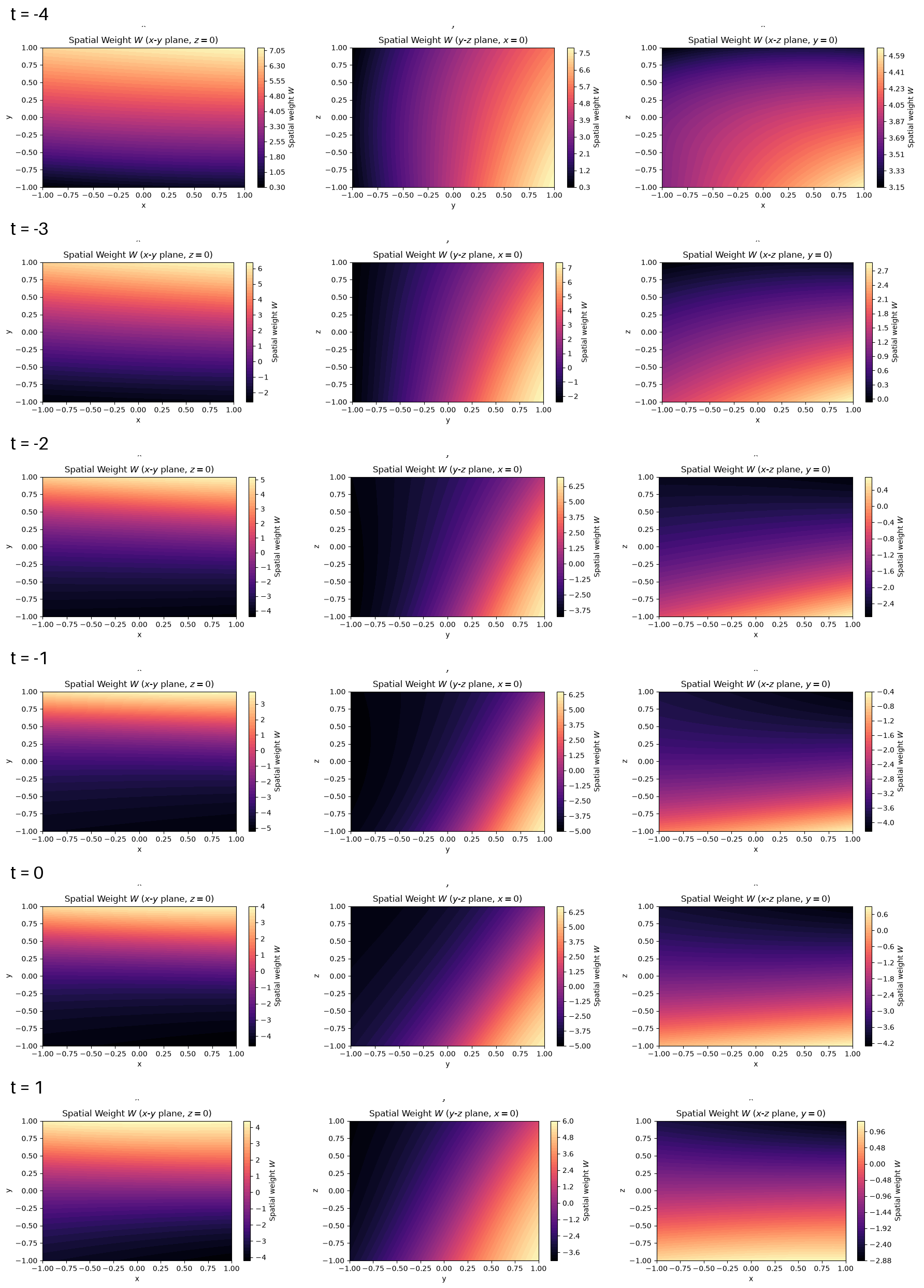
At the best checkpoint, $W$ is still high at the boundary, but from $t = -3$ onwards it’s negative across large parts of space, down to about $-5$, and about zero at the observer today. Negative $W$ weights the physics up.
That’s when the expansion took off. While the physics was turned down, $H$ today crept up to 14% of $H_0$ and stalled for six thousand steps. Between the two times I looked at $W$, the field-equation residual fell more than fiftyfold, and $H$ climbed from 14% to 45%. With the field equations finally carrying weight, the Friedmann constraint did what it had been asking for all along, and expansion took over from curvature in balancing the matter.
The forbidden rise in $H(t)$ tracks it too. At step 10,000 the peak was more than five times the boundary rate. At the best checkpoint it’s 1.9 times. The more weight the field equations get, the less of the stretch that dust can’t produce is left.
And then it fell apart Link to heading
After step 40,000 the run came apart. The supernova fit got worse, rays stopped reaching every source, and $H$ gave back most of what it had gained, falling to 14% of $H_0$ by the end. There was no new best after step 38,023.
I don’t know why yet. The loss has single-step spikes, up to fifteen million, which points at the energy condition’s enormous multiplier, now over 170,000, landing on points where $W$ is low. But they were just as frequent during the good stretch, so they don’t explain the turn.
Why we didn’t see it sooner Link to heading
For this to bite, something has to pull against the physics. Until part 5, the supernova data never reached the network, so there was nothing to trade a violation against and no reason to hide one. This is the first run where the data and the physics genuinely compete. It’s also the first time I’ve looked at $W$, so I don’t know how far down it had turned the physics in parts 3 to 5.
What’s next Link to heading
The energy condition, outside the weighting Link to heading
The energy condition’s penalty comes out of the spatial weighting and sits beside the CMB constraints, where its weight and multiplier mean what they say. The field equations stay inside the weighting for now.
This run makes a prediction for the next one. Without the energy condition inside it, $L$ at each point is just the field-equation residual, so $W$ should go below zero from the start and weight the field equations up straight away. It took this run thirty thousand steps to get there by accident. If $W$ stays high, I’ve got the mechanism wrong, and the weighting comes off the field equations too.
Holding $H$ to what we measure Link to heading
Even at its best, $H$ reached 45% of $H_0$, and it didn’t stay there. So after the energy condition, the expansion band from part 5 goes in: $H$ between 60 and 80 km s⁻¹ Mpc⁻¹, as a Lagrangian constraint like the others.
It applies at one point: the observer, today. That follows from what SH0ES actually measures, which is the slope of redshift against distance for supernovae in every direction on the sky. For nearby sources, in any spacetime, that slope is
$$cz \approx d\,\left(\tfrac{\theta}{3} + \sigma_{ij} n^i n^j\right)$$evaluated at the observer (Kristian & Sachs, 1966). The shear term is a quadrupole on the sky and averages away over directions, leaving $\theta/3$: the local expansion rate at the observer’s own position. No homogeneity is assumed anywhere in that.
Constraining an average over a volume would assume something. It would equate the measured $H_0$ with the volume-averaged expansion rate, and in a lumpy universe those differ. The difference is backreaction, which is exactly what this project is trying to measure.
The rest of space is left alone. A locally expanding region around the observer is a legitimate inhomogeneous answer (void models are one of the classic alternatives to dark energy), and the supernovae across the light cone still have to fit whatever the network builds.
Once $H$ at the observer is held at the measured rate, matter can supply about 29% of $3H^2$ there. Whatever combination of shear and negative spatial curvature the network uses for the other 71% is the answer to the question this project started with.